Support Vector Machines

`# General Idea

SVMs retains three attractive properties:

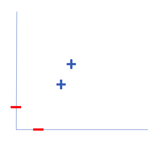
1. SVMs construct a maximum margin separator - a decision boundary with the largest possible distance to example points, helping to generalise well.
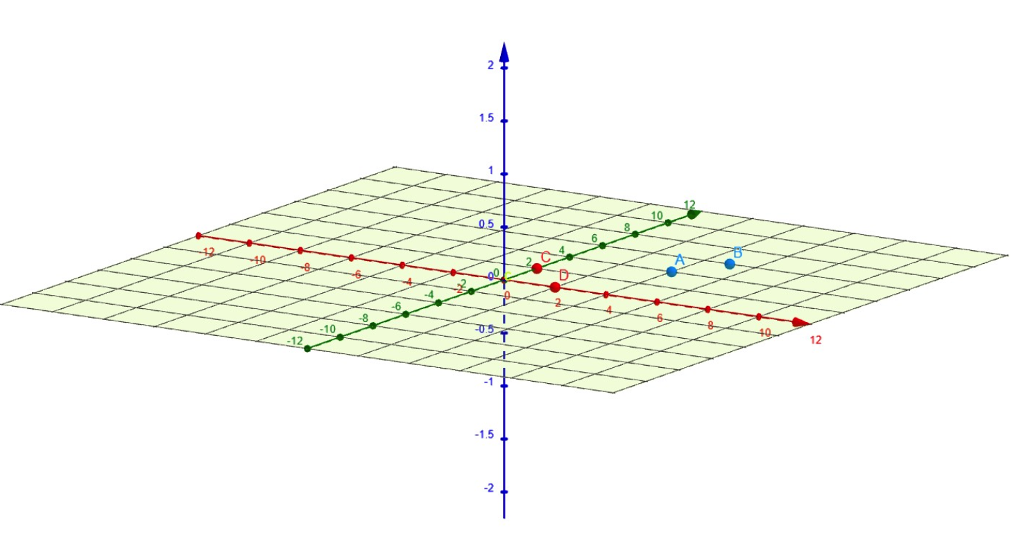
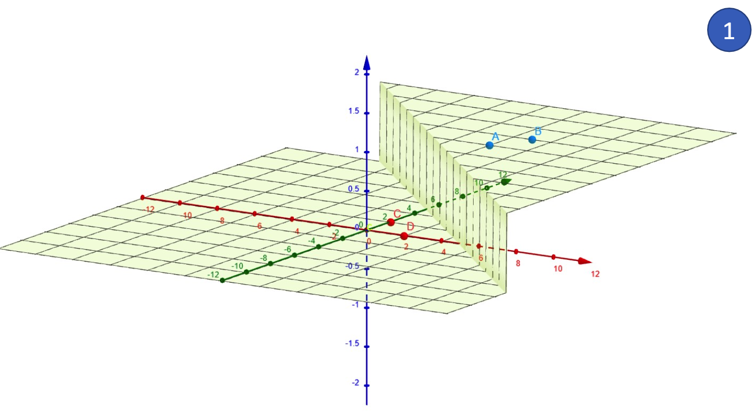
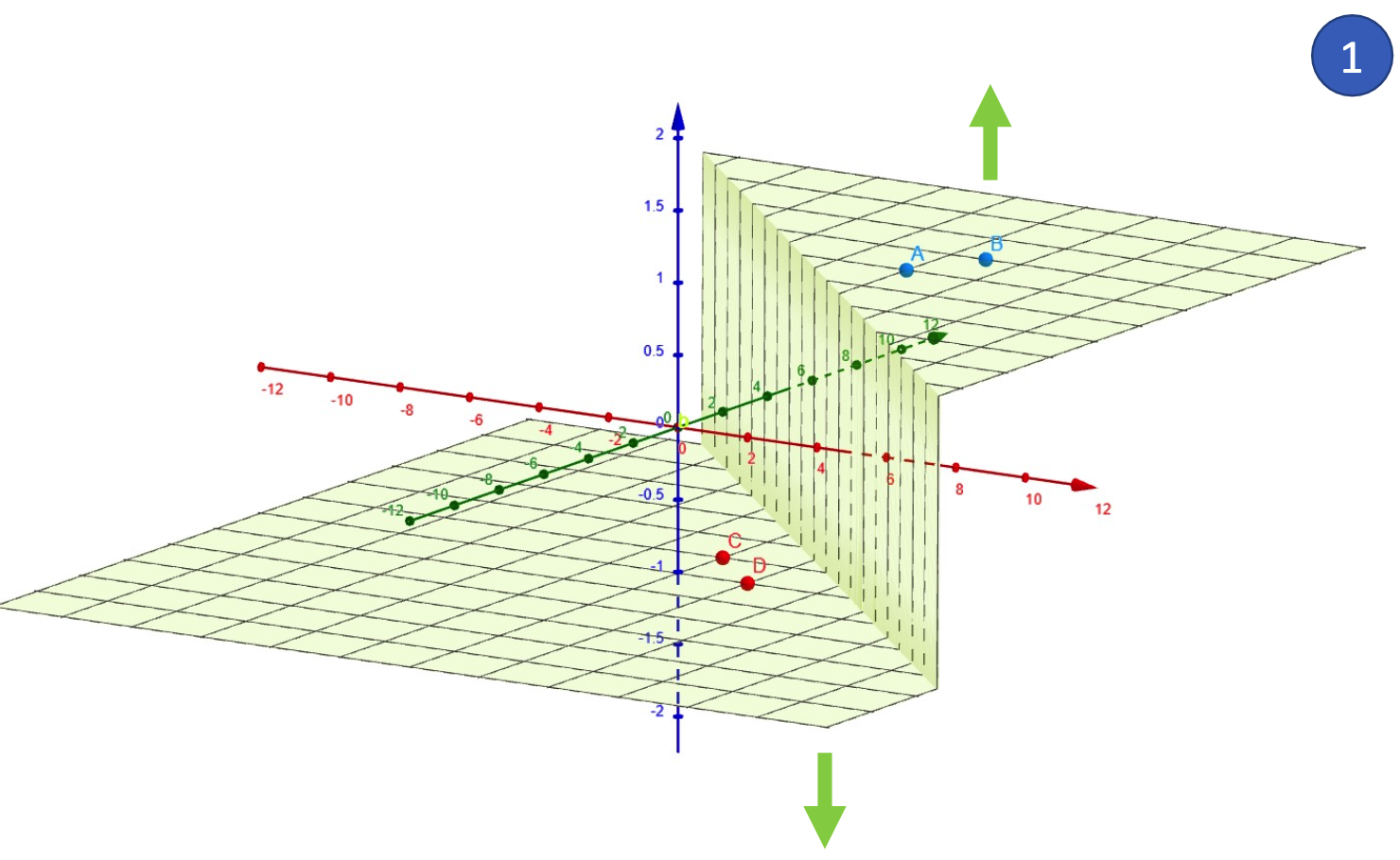
2. SVMs create a linear separating hyperplane, allowing data that are not linearly separable in the original input space to be easily separable in the higher dimensional space.
3. SVMs are non-parametric - instead of learning a fixed number of parameters like in logistic regression or neural networks, SVMs define the decision boundary using only a subset of training points (the support vectors). However, it only keeps the examples closes to the separating plane, generalizing well like parametric models, and retaining flexibility like non-parametric models.

To maximise the margin,

1. define the appropriate decision rule
2. define margin, and find equation for it
3. derive optimisation problem that maximises margin while being consistent with data

Step 1: Decision rule, given weights , vector , and bias :

Step 2: Equation for the margin

The margin is the distance between the support vectors, which represent the closest points to the decision boundary. The margin is inversely proportional to the norm of , thus maximising the margin would mean minimising .

Step 3: Constrained optimization problem

The optimisation problem maximises the margin - while ensuring all points are classified correctly with the constraint .

Summary

• Classifier with optimal decision boundary

Hyperplanes

Hyperplane

The zero-offset hyperplane is defined by a normal vector and contains all vectors for which

With the sign of , we can find the side a point is with respect to the zero-offset hyperplane.

For example, given the weights and the point ,

we can find that

• the point lies on the positive side of the hyperplane ()
• the distance from the point to the hyperplane:

Objective

Given data points, with each consisting of

• features , described in a vector of real numbers in dimension
• target variable

The SVM classifier in the dual formulation is a model that depends on parameters .

Sparsity

Generally, many of the points , as only a few data points are exactly on the margin. These data points are the support vectors.

Hard-Margin SVM (Linearly Separable)

The assumption for this section is that the data is linearly separable

Given labeled data of two classes , the data is preprocessed such that:

For notations, a data point of class is indicated as and a data point of class is indicated as .

Step 1: Decision Rule

where

Considering the constraints for existing data:

Thus,

The equality constraint, thus, is satisfied from the following:

and thus, if the lies on the margin:

satisfying the equality constraint, which is crucial as

• it identifies support vectors - the subset of training points that determine the position and orientation of decision boundary
• which is used for computing the optimal hyperplane

Step 2: Margin Equation

Given that we have the decision rule, we can then find the margin equation:

Step 3: Maximising Margin

Thus, we can maximise the margin (indicated in blue) while classifying correctly (indicated in yellow).

Thus, we get the constrained optimisation problem, where we minimise , , to maximise the margin.

subject to the constraint as mentioned above.

To solve this, Lagrange multipliers are introduced for each data point:

to convert the constrained optimisation problem into an unconstrained one. The term insides the summation instead, enforces the classification constraint.

Effectively, we are trying to maximise the Lagrangian multiplier, while minimising the weights and bias of the margin, getting the optimisation problem:

We can then solve the optimisation problem, first by (partially) differentiating with regards to :

This means only support vectors (points where the Lagrangian multiplier ) define , making computation efficient.

then, we (partially) differentiate with regards to :

This ensures that the classifier is balanced around the decision boundary.

We then can plug these back into the Lagrange function to achieve the dual objective:

To get the maximum of , it becomes a quadratic optimisation problem which can be solved by Quadratic Programming (QP) solvers.

Soft Margin SVM (Non-Linearly Separable)

However, the data might not be linearly separable. If the data is non-linearly separable, a standard linear SVM won’t work because a straight hyperplane cannot separate the classes.

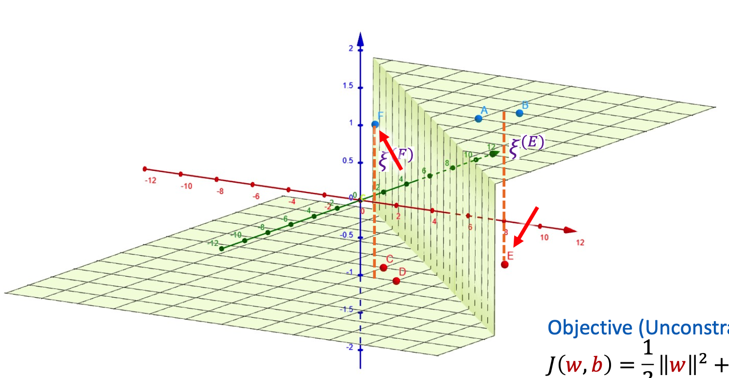
Introducing Slack Variables

With slack variables, we allow for some slack variables to allow some misclassifications:

New Objective Function

With this, the new optimisation problem becomes,

where

The unconstrained objective function then becomes: